View

The View option offers three possibilities. Figures can be exported in various formats (EPS, JPEG, etc.).

1- Histogram

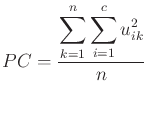
Distribution of values, displayed together with the fuzzy partition, if there is a current FIS. Two indices are displayed below each partition: the partition coefficient, $PC$,to be maximized, and the entropy coefficient, $PE$, to be minimized.

In the formulae below, $c$ is the number of MFs, $n$ the number of rows in the dataset and $u_{ik}$ is the membership of example $k$ in the $ith$ MF.

$$PC =\frac{\displaystyle\sum_{k=1}^n \sum_{i=1}^c u^2_{ik}}{n}$$

$$PE = - \frac1n \left\{\sum_{k=1}^n \sum_{i=1}^c \left[u_{ik} \log_a (u_{ik})\right]\right\}.$$

2 - X-Y graph

On the 2 variable plot, options allow to display the regression line, or the axis bisector.

The left click on a data point activates/deactivates it, with a dynamical link to the data table presented below. In case of a graphical difficulty to identify the point, it may be easier to activate/deactivate it from the data table, which has checkboxes for that purpose.

An info balloon shows the row number of the data point near the mouse location.

3 - X-Y-Z graph

The points corresponding to the chosen variables are displayed on a 3D graphics.

The same functionalities than for the 2D plot are available, plus some other mouse actions:

• Press left button + move: rotation
• Press right button + move: translation
• Press wheel + move: zoom.

The  Reset view option of the File menu resets the 3D graph to its initial values.