Next: Rule induction Up: Partitions Previous: Generate a FIS without Contents
The HFP method, which means Hierarchical Fuzzy Partitioning is described in detail in [9,10].
It includes a fuzzy partitioning stage and a rule selection one.
We only present here the four steps proposed in the menu. A current data file must be available.
The k-means option uses the well known clustering method of the same name. There is no a priori relationship, for a given variable, between the partition centers for partitions of different sizes.
This last option corresponds to an ascending procedure. At each step, for each given variable, two fuzzy sets are merged. The computational time can be high, and essentially depends on the initial number of fuzzy sets. There are two ways to build the initial partition. The first one consists of considering the values in the learning set as identical if they differ by less than the threshold (given as a percentage of the input range). Each group of values, the number of groups depending on that threshold, then corresponds to one fuzzy set. The second way sets the number of groups, and calculates the group centers by applying a k-means clustering.
This option creates a file that records the vertex coordinates for all proposed partitions. The partition size goes from two to the maximum number (default is 7) set at step 1.
This option is for viewing the vertex location, together with the data distribution (histogram).
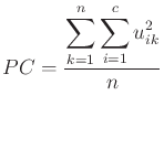
Two indices are displayed below each partition: the partition coefficient, ![]() ,to be maximized, and the entropy coefficient,
,to be maximized, and the entropy coefficient, ![]() , to be minimized.
, to be minimized.
In the formulae below, ![]() is the number of MFs,
is the number of MFs, ![]() the number of rows in the dataset and
the number of rows in the dataset and ![]() is the membership of example
is the membership of example ![]() in the
in the ![]() MF.
MF.
![$\displaystyle PE = - \frac1n \left\{\sum_{k=1}^n \sum_{i=1}^c \left[u_{ik} \log_a (u_{ik})\right]\right\}.$](img20.png)
The one-dimensional hierarchies calculated at step 1 are used to build fuzzy inference systems. It is an iterative procedure which starts from a 1 or 2 fuzzy set partition for each input dimension, builds the fuzzy inference system including all possible rules and assigns it performance and coverage indices. At each iteration, a single input variable fuzzy partition is refined by adding one fuzzy set, and the corresponding fuzzy inference system is built. The best fuzzy inference system will be kept considering the performance criterion. The procedure uses a HFP configuration file and a vertex file. The first five parameters are identical to those described in the Generate Conclusions Menu (fpa algorithm). The next one corresponds to the initial number of fuzzy sets in the partition. It can be set to 1 or 2. The default value is 1, and corresponds to introducing variables one by one.
The last two parameters allow to set a maximum number of iterations, and to specify a validation file for evaluating the FIS performance. The default validation file is the current data file. Other files can be used, in particular the active or inactive data file created by the use of the Data-table menu option.
Output files:
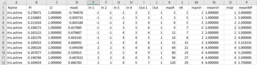
The results of each iteration are stored as a line in both files "result" and "result.min". The "result" file records all attempts (adding a fuzzy set on each input variable), and the "result.min" file holds the configuration retained after each iteration.
Format: columns are delimited by the & character, which allows easy import into a spreadsheet, or immediate introduction as an array in a LaTeX document.
The performance and coverage indices are described in part II,section 2, while the rule base characteristics are introduced in section 3,part II.
Output file analysis allows the user to select one or more FIS to generate. Elements to be considered are the performance (column 6) and the coverage level (column 4) but also the complexity of each FIS, which is measured by the number of rules (column 3),and other rule base characteristics provided by the InfoRB structure.
The performance index, which is an error measure, should be as small as possible (minimum 0), and the coverage level as high as possible (maximum ![]() ), while the number of rules and of fuzzy sets must be kept reasonably small.
The compromise between complexity and accuracy is under user control.
), while the number of rules and of fuzzy sets must be kept reasonably small.
The compromise between complexity and accuracy is under user control.
Note: This option does not generate a FIS.
This option, available in the Rule Induction-HFP FIS option, creates a FIS configuration file for a given combination.
The HFP configuration file and the vertex file are given as parameters. The other parameters are used to initialize the rule conclusions using the FPA algorithm. The generated FIS can be used as such, or as an input to the simplification menu.